
Lookups, and the argument everyone leaves off
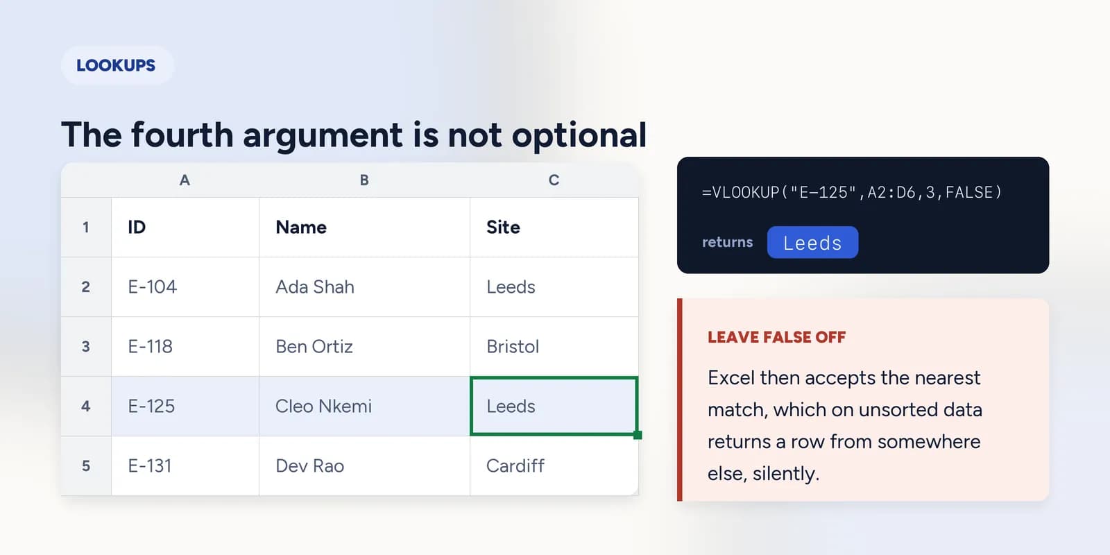
VLOOKUP finds a row by the value in the table's first column and reads across to a column you number: =VLOOKUP("E-125", A2:D6, 2, FALSE). The fourth argument is the one that matters. FALSE demands an exact match; leaving it off tells Excel to accept the nearest match, which on unsorted data returns a row from somewhere else without any error at all.

A lookup answers the question you actually have about a table: I know this one thing about a row, tell me something else about it. It is where most real spreadsheet work happens, and VLOOKUP is still the function most people reach for.
It also has a default that is dangerous, and that is what most of this page is about. Three of VLOOKUP's four arguments are obvious. The fourth decides whether a wrong answer arrives as an error you can see or as a number you believe.
VLOOKUP, and the fourth argument
VLOOKUP takes what you are looking for, the table to look in, which column to read out counting from the left of that table, and whether you want an exact match. The column is a number, not a letter, and it counts from the start of the range rather than from column A of the sheet.
| A | B | C | D | |
|---|---|---|---|---|
| 1 | ID | Name | Site | Salary |
| 2 | E-104 | Ada Shah | Leeds | 41000 |
| 3 | E-118 | Ben Ortiz | Bristol | 38500 |
| 4 | E-125 | Cleo Nkemi | Leeds | 52000 |
| 5 | E-131 | Dev Rao | Cardiff | 44750 |
| 6 | E-147 | Eli Fontes | Bristol | 36200 |
=VLOOKUP("E-125",A2:D6,3,FALSE)Column 3 of the range, counting A as 1. FALSE means an exact match or nothing.
There is exactly one case where TRUE is the right answer: a banded lookup, where you have thresholds in ascending order and you genuinely want the band a value falls into. Commission tiers and tax bands work this way. Everything else wants FALSE.
What #N/A and #REF! are each telling you
The two errors a lookup produces mean completely different things, and knowing which is which turns a mystery into a two-minute fix.
- #N/A means the value was not found. The lookup itself is well-formed. Either it genuinely is not there, or the two values differ invisibly: a trailing space, or a code stored as text on one side and as a number on the other.
- #REF! means the column number is outside the range. Asking for column 5 of a four-column table produces it, and so does deleting a column that the formula was counting on.
- A wrong answer with no error at all usually means the fourth argument was left off.
IFNA is the right wrapper for a lookup you expect to miss sometimes, because it catches only #N/A and leaves a genuine #REF! visible. IFERROR hides both, which turns a broken formula into a tidy-looking blank.
XLOOKUP, and what it fixes
XLOOKUP takes two separate ranges rather than one table and a column number: where to look, and what to return. That removes the counting, removes the fragility, and removes the limitation that VLOOKUP can only read to the right of the column it searched.
=XLOOKUP("E-131",A2:A6,C2:C6)Look in the ID column, return from the site column. Exact match is the default rather than something to ask for.
- No column number, so inserting a column into the table cannot silently change what the formula returns.
- Exact match by default, so the dangerous case has to be chosen deliberately.
- It can return a value from a column to the left of the one it searched, which VLOOKUP cannot.
- A fourth argument supplies a message for when nothing is found, instead of #N/A.
INDEX and MATCH, the portable version
MATCH tells you the position of a value in a range. INDEX returns what is at a given position. Put one inside the other and you have a lookup that works in any direction and in any version of Excel.
=INDEX(B2:B6,MATCH("E-147",A2:A6,0))MATCH finds which row holds E-147, INDEX reads the name at that position. The 0 in MATCH is what makes it an exact match.
It reads awkwardly the first few times, and the payoff is that the two ranges are independent. Insert a column anywhere, read leftwards, point the two halves at different sheets: none of it breaks the formula, because nothing in it is counting columns.
What goes wrong
These are the mistakes this part exists to prevent. Each one is reasonable, which is why people make it and why nothing on the sheet objects.
Leaving the fourth argument off VLOOKUP
WhyIt is marked optional, and on a sorted table it often returns the right answer anyway, which teaches the wrong lesson.
InsteadAlways write FALSE unless you are deliberately doing a banded lookup. The default is approximate matching, which fails silently.
Counting the column from column A of the sheet
WhyColumn letters are right there along the top, and the number in the formula looks like it should correspond to them.
InsteadCount from the first column of the range you gave the function. If the table starts at C, then C is column 1.
Wrapping a lookup in IFERROR to tidy it up
WhyIt makes an ugly column of #N/A disappear, and the sheet immediately looks finished.
InsteadUse IFNA, which catches only not-found. IFERROR also swallows #REF! and #VALUE!, so a formula that has genuinely broken keeps reporting the friendly message you wrote.
Common questions
How do I use VLOOKUP in Excel?
=VLOOKUP(what you are looking for, the table, which column to read counting from the left of that table, FALSE). The value you search for must be in the table's first column.
Why does my VLOOKUP return #N/A?
The value was not found. Usually that means a trailing space on one side, or a code stored as text in one column and as a number in the other. Wrap the lookup value in TRIM and compare ISNUMBER on both columns.
What is the difference between VLOOKUP and XLOOKUP?
XLOOKUP takes separate lookup and return ranges instead of a column number, defaults to exact match, can return values to the left, and has a built-in not-found message. It needs Microsoft 365 or Excel 2021.
Is INDEX MATCH better than VLOOKUP?
It is more robust: it can look in any direction and does not break when a column is inserted. XLOOKUP is easier to read and does the same things, so INDEX MATCH is mainly for workbooks that must run on older Excel.
Can VLOOKUP look to the left?
No. It only ever reads columns to the right of the one it searched. Use XLOOKUP, or INDEX with MATCH, when the answer sits to the left of the key.